

Gandalf Oracles – Asset Allocation
Aggiornamento Live Trading – 25 Settimane · Settembre 2025 – Febbraio 2026
Gandalf Oracles – Asset Allocation
Live Trading Update – 25 Weeks · September 2025 – February 2026
Prima di lasciarvi all’interessante analisi di Francesco Federici (uno dei nostri architetti di strategie quantitative ed AI-driven che alimentano i Gandalf Oracles), desidero fare un paio di premesse.
Da novembre 2024, anche grazie al lavoro fatto insieme a Michael Trequattrini (architetto di strategie e Quantitative Researcher), abbiamo lanciato il Volatility Forecaster (consultate la nostra sezione articoli per approfondimenti), una previsione settimanale della volatilità futura dei 100 asset a maggiore capitalizzazione dell’S&P500. Da allora, ogni settimana, un insieme di modelli di AI, alimentati da dataset differenti, concorre a creare un’unica predizione di sintesi per ciascuno degli asset per la settimana successiva (questa informazione è ad oggi gratuita e per riceverla è sufficiente scrivere ad info@gandalfproject.com). Questo dato può essere uno strumento estremamente utile e versatile in svariate applicazioni finanziarie, dalla composizione di portafogli di asset allocation, fino all’operatività in opzioni (dove si può comprare e vendere volatilità).
Il Volatility Forecaster costituisce il primo “oracolo” dei Gandalf Oracles, che oggi non predicono più soltanto la volatilità, ma anche la direzione (va detto con un’incertezza maggiore), il ranking di forza relativa e gli scenari di mercato su diversi orizzonti temporali. Proprio grazie ad una ricerca costante e meticolosa, stiamo lavorando per rendere questi strumenti davvero competitivi e, per farlo, li abbiamo allestiti in modo centralizzato, approvvigionando i nostri agenti con pletore di strategie eterogenee che controlliamo da quando nascono a quando muoiono. Alcune di queste strategie derivano dal Machine Learning più tradizionale (Ensemble Methods, Deep Neural Networks, Spiking Neural Networks ecc.), altre hanno matrice genetica (Genetic Asset Management), altre ancora derivano dal Reinforcement Learning o dal Generative AI.
La chiave è che oggi è possibile ideare e realizzare una elevata diversificazione, gestendo i singoli modelli concorrenti, monitorandone la qualità nel tempo e conservando un controllo diretto su ciascuno di essi.
L’apparente mancanza di limitazioni (oggi con gli LLM si può passare da un paper accademico ad un codice operativo in modo rapido) e la potente scalabilità (non solo numerica) dei modelli sintetizzati, deve tuttavia fare i conti con gli stessi demoni di sempre: la de-correlazione dei modelli, la liquidità degli strumenti di applicazione ed i costi di esercizio delle strategie finali.
Di seguito Francesco Federici ci aggiorna sulle performance reali di uno di questi agenti, in monitoring e sul mercato da settembre 2025.
Non mi dilungo ulteriormente e vi lascio alla lettura
Giovanni Trombetta
Head of R&D
Gandalf Project
Gandalf Oracles – Asset Allocation
Aggiornamento Live Trading – 25 Settimane
Settembre 2025 – Febbraio 2026
“Si può guadagnare se il mercato non sale?”
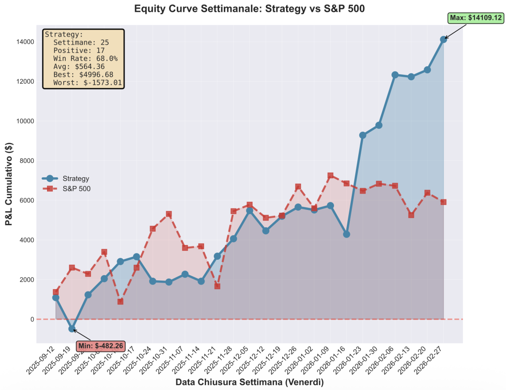
Questa è la domanda che ci siamo posti e a cui il mercato sta, in parte, rispondendo per noi. Nelle ultime tre settimane l’S&P 500 è passato da +6.73% a +5.91% rispetto all’inizio del nostro track record.
È sceso.
Il benchmark che tutti seguono ha restituito una parte dei guadagni. E la nostra strategia? È passata da +12.33% a +14.11%.
Ha subito un’ulteriore accelerazione.
Questo aggiornamento, a 25 settimane, racconta esattamente questo: cosa succede quando il mercato si ferma, torna indietro, diventa laterale ed un sistema sembra in grado di continuare a generare alpha.
1. Il Paradosso: Mercato Piatto, Strategia in Accelerazione
Chi opera sui mercati sa bene che la maggior parte delle strategie long-only vive e muore con il benchmark. Se l’S&P sale, tutti festeggiano. Se scende o rimane laterale, i portafogli soffrono. È la realtà dei beta player: esposti al mercato, dipendenti dalla sua direzione.
I Gandalf Oracles cercano di giocare ad un’altra partita. E le ultime 3 settimane di operatività lo hanno dimostrato in modo ancora più evidente di prima (sappiamo bene come questo non sia ancora sufficiente, ma costituisca comunque un primo segnale da monitorare).
Evoluzione delle Metriche Chiave
| Metrica | Report 7 Feb | Report 28 Feb | Variazione |
|---|---|---|---|
| Return Strategy | +12.33% | +14.11% | +1.78% |
| Return S&P 500 | +6.73% | +5.91% | -0.82% |
| Outperformance | +5.60% | +8.20% | +2.60% |
| Sharpe Ratio | 2.21 | 2.30 | +0.09 |
| N° Trade | 141 | 158 | +17 |
| Win Rate | 55.3% | 56.3% | +1.0% |
| P&L Totale | $12,326 | $14,109 | +$1,783 |
Mentre il benchmark ha ceduto quasi un punto percentuale (-0.82%), la strategia ha aggiunto quasi 2 punti (+1.78%). Il gap di outperformance è esploso da +5.60% a +8.20%. E lo Sharpe è salito a 2.30. In un momento in cui il mercato arretra, la nostra efficienza risk-adjusted migliora.
Il mercato scende, la strategia accelera. L’outperformance è più che raddoppiata in 3 settimane: da +5.60% a +8.20%. Questo non è semplice esposizione direzionale al mercato. È una componente di rendimento che, nel modello adottato, non risulta spiegata dal beta.
2. Perché Funziona Quando il Mercato Non Si Muove?
La risposta sta in tre numeri che raccontano una storia piuttosto chiara:
β = 0.11
Beta contenuto – Bassa esposizione direzionale al mercato
| Metrica | Valore | Interpretazione |
|---|---|---|
| Beta | 0.11 | Indica una bassa esposizione direzionale al mercato. |
| Correlazione | 0.13 | Indica un co-movimento molto contenuto con l’S&P 500 nel campione osservato. |
| R-Squared | 0.016 | Solo l’1.6% della varianza dei rendimenti è spiegata dal mercato nel modello lineare utilizzato. |
| Alpha (ann.) | +18.73% | Indica che, nel campione analizzato e secondo il modello lineare utilizzato, il rendimento non è spiegato dall’esposizione al mercato. |
| Convexity | +20.88 | Evidenzia una componente non lineare positiva nel campione osservato. |
Alpha +18.73%
Indica che, nel campione analizzato e secondo il modello lineare utilizzato, il rendimento non è spiegato dall’esposizione al mercato, ma dalla capacità dell’agente nel selezionare le baseline corrette.
Convexity +20.88
Il valore stimato indica la presenza, nel campione osservato, di una componente non lineare positiva nella relazione con il mercato. In termini semplici, la strategia mostra una sensibilità che non è puramente lineare: la risposta ai movimenti dell’indice non cresce in modo proporzionale, ma evidenzia una dinamica più articolata.
La regressione con termine quadratico suggerisce quindi una possibile risposta asimmetrica ai movimenti di mercato, pur trattandosi di una strategia long-only, senza utilizzo di derivati, leva finanziaria o posizioni short.
LOW BETA PROFILE CON SOLO POSIZIONI LONG: con un R² pari a 0.016, solo l’1.6% della varianza dei rendimenti è spiegata dal benchmark nel modello lineare adottato. La gran parte della variabilità osservata non risulta attribuibile al mercato, caratteristica che può renderla interessante in ottica di diversificazione di portafoglio.
3. Confronto Completo: Strategy vs S&P 500 a 25 Settimane
Dopo 25 settimane di operatività live, 158 trade eseguiti autonomamente, il quadro complessivo si è rafforzato su tutti i fronti:
| Metrica | Strategy | S&P 500 | Delta |
|---|---|---|---|
| Total Return | +14.11% | +5.91% | +8.20% |
| Max Drawdown | -2.70% | -5.11% | +2.41% |
| Sharpe Ratio | 2.30 | 0.91 | +1.39 |
| Sortino Ratio | 1.24 | 0.96 | +0.27 |
| Calmar Ratio | 5.22 | 1.16 | +4.06 |
| Volatility (ann.) | 8.55% | 9.72% | -1.17% |
| Win Rate | 56.33% | — | — |
| Profit Factor | 1.56 | — | — |
Le metriche sono calcolate su un campione di 25 settimane; la stabilità dei parametri nel tempo richiede validazione su orizzonti più lunghi e differenti regimi di mercato.
Osserviamo il Calmar Ratio (non annualizzato sul periodo di test): 5.22 contro 1.16. Significa che per ogni punto di drawdown massimo sopportato, la strategia ha generato 5.22 punti di rendimento. L’S&P 500 ne genera poco più di uno. Il Calmar è forse una delle metriche più esplicite quando si opera: ti dice quanto dolore devi sopportare per ogni unità di guadagno. Il nostro è 4.5 volte quello del benchmark.
E la volatilità? La strategia ha una volatilità annualizzata dell’8.55%, contro il 9.72% del benchmark. Rendiamo di più, rischiando di meno. Stando ai 158 trade documentati fino ad oggi, con i prezzi reali di Interactive Brokers.
4. Performance Settimanale: Dove Si Nasconde la Consistenza
25 settimane di operatività. 17 positive, 8 negative. Un Win Rate settimanale del 68% che racconta di un sistema che non vince per un colpo fortunato, ma per accumulo sistematico.
| Metrica Settimanale | Valore |
|---|---|
| Settimane Operative | 25 |
| Settimane Positive | 17 (68.0%) |
| P&L Medio per Settimana | $564.36 |
| Miglior Settimana | $4,996.68 (w/e 23 Gen) |
| Peggior Settimana | -$1,573.01 (w/e 19 Set) |
| P&L Medio Trade | $89.30 |
| Commissioni Totali | $374.02 ($2.37/trade) |
La miglior settimana (+$4,997) vale 3.2 volte la peggior settimana (-$1,573). È l’asimmetria favorevole in azione: quando guadagnamo, guadagnamo di più. Quando perdiamo, le perdite sono contenute. Questa caratteristica è il riflesso diretto della convexity positiva che emerge dall’analisi della correlazione.
Le ultime 3 settimane aggiunte sono state: -$97 (settimana debole ma controllata), +$351, +$1,530. Due su tre positive, con l’ultima che ha compensato la prima settimana negativa di un fattore 16x. È così che si accumula alpha: non evitando le perdite, ma compensandole con guadagni asimmetrici.
5. Top e Bottom Performer: La Selezione Conta
L’analisi per ticker rivela come il motore di selezione distribuisce il rischio e cattura le opportunità:
Top 5 Performer
| Simbolo | P&L ($) | N° Trade | Win Rate | Settore |
|---|---|---|---|---|
| TJX | +$6,827 | 10 | 80.0% | Consumer Disc. |
| LLY | +$3,657 | 4 | 50.0% | Health Care |
| EQT | +$2,743 | 10 | 70.0% | Energy |
| ACGL | +$2,131 | 12 | 66.7% | Financials |
| GILD | +$1,985 | 9 | 77.8% | Health Care |
Bottom 5 Performer
| Simbolo | P&L ($) | N° Trade | Win Rate | Settore |
|---|---|---|---|---|
| INTU | -$3,726 | 10 | 40.0% | Technology |
| NEM | -$1,511 | 4 | 50.0% | Materials |
| ROP | -$844 | 4 | 50.0% | Technology |
| MSFT | -$360 | 2 | 50.0% | Technology |
| NVDA | -$210 | 9 | 44.4% | Technology |
TJX resta il leader assoluto con quasi $7,000 di profitto e un win rate dell’80% su 10 trade. Il dato interessante è la diversificazione settoriale dei top performer: Consumer Discretionary, Health Care, Energy, Financials. Non c’è concentrazione su un singolo settore di mercato.
Sul fronte negativo, INTU (Intuit) continua a pesare con -$3,726. Ma il dato chiave è che la somma dei top 5 (+$17,343) supera di gran lunga la somma dei bottom 5 (-$6,651). Il rapporto guadagni/perdite dei migliori vs peggiori è quasi 3:1. Il sistema è in grado di generare alpha.
6. Aggiornamento Slippage: Broker vs Teorico
Nell’articolo precedente avevamo documentato uno dei risultati più contro-intuitivi: lo slippage positivo, il P&L reale che superava quello teorico calcolato sui prezzi Yahoo Finance. Con 3 settimane di dati in più, il quadro si è aggiornato:
| Metrica Slippage | Report 7 Feb | Report 28 Feb |
|---|---|---|
| P&L Reale (Broker) | $12,326.04 | $14,109.12 |
| P&L Teorico (Yahoo) | $11,767.95 | $15,065.10 |
| Differenza | +$558.10 (+4.74%) | -$955.98 (-6.35%) |
| Media Diff. per Trade | +$3.96 | -$6.05 |
Il dato è cambiato: lo slippage è passato da leggermente positivo a leggermente negativo. Questo è più in linea con le aspettative teoriche, nella realtà operativa, è normale aspettarsi un certo costo di esecuzione. Tuttavia, -$6.05 per trade è un valore assolutamente contenuto, specialmente considerando che il P&L medio per trade è di $89.30.
Lo slippage rappresenta circa il 6.8% del P&L medio, un costo di esecuzione irrisorio che conferma la qualità dell’infrastruttura MOO/MOC su Interactive Brokers. Il confronto con Yahoo Finance rimane comunque imperfetto: i prezzi di riferimento differiscono strutturalmente dagli execution price delle aste, e la variabilità trade-by-trade (64 migliori vs 94 peggiori) è fisiologica.
Lo slippage normalizzato (-6.35%) è contenuto e non compromette il profilo di alpha della strategia. Il costo di esecuzione reale è marginale rispetto al rendimento generato.
7. Cosa ci stanno dicendo i Dati
25 settimane. 158 trade. Zero intervento umano. E un messaggio che diventa sempre più chiaro man mano che il track record si allunga:
Non serve che il mercato salga per guadagnare.
Il lavoro che stiamo facendo con i Gandalf Oracles sta dimostrato nei fatti, non in simulazione, che un sistema AI-driven di asset allocation settimanale può generare alpha indipendente dalla direzione del mercato. Con un Beta di 0.11 e un Alpha annualizzato del +18.73%, il sistema rappresenta un caso di studio nel panorama delle strategie quantitative.
Le ultime 3 settimane hanno offerto la dimostrazione più elegante: il benchmark arretra, l’outperformance si allarga, lo Sharpe sale. È esattamente il comportamento che ci si aspetta da una strategia genuinamente decorrelata con il mercato su cui viene applicata.
Naturalmente, 25 settimane restano un campione limitato e le performance passate non sono indicative di risultati futuri. Ma la coerenza tra le previsioni teoriche dell’architettura (decorrelazione, convexity, alpha puro) e i risultati effettivi è un segnale forte. L’agente non sta facendo qualcosa di diverso da ciò per cui è stato progettato, lo sta facendo in modo consistente, trade dopo trade, settimana dopo settimana.
Continueremo a documentare ogni aspetto di questo percorso con la trasparenza che lo ha caratterizzato fin dall’inizio.
Buon trading!
Francesco Federici
R&D Team – Gandalf Project
Febbraio 2026
Avvertenza importante — Non è consulenza finanziaria
Importante: né questo articolo né i tool, i modelli o gli agenti citati nell’articolo forniscono consulenza finanziaria, consulenza di investimento, raccomandazioni di trading o qualsiasi altro tipo di servizio finanziario regolamentato.
Tutti i contenuti, i dati, gli esempi operativi, le metriche e le analisi presentate sono esclusivamente a scopo informativo e non costituiscono in alcun modo un invito a comprare, vendere o detenere strumenti finanziari.
Le performance passate, i risultati osservati e i pattern storici non rappresentano una garanzia di risultati futuri. Ogni decisione di investimento deve essere presa in modo autonomo e, se necessario, con il supporto di un consulente finanziario qualificato.
Il trading e l’investimento comportano rischi significativi, inclusa la possibile perdita del capitale investito.
Before leaving you to Francesco Federici’s interesting analysis (one of our architects of quantitative and AI-driven strategies powering the Gandalf Oracles), I would like to make a couple of preliminary remarks.
Since November 2024, also thanks to the work carried out together with Michael Trequattrini (strategy architect and Quantitative Researcher), we have launched the Volatility Forecaster (please refer to our articles section for further details), a weekly forecast of the future volatility of the 100 largest-cap assets in the S&P 500. Since then, every week, a set of AI models, fed by different datasets, contributes to creating a single synthetic prediction for each asset for the following week (this information is currently free and, to receive it, you simply need to write to info@gandalfproject.com). This data can be an extremely useful and versatile tool in a wide range of financial applications, from asset allocation portfolio construction to options trading (where volatility can be bought and sold).
The Volatility Forecaster is the first “oracle” of the Gandalf Oracles, which today no longer predict only volatility, but also direction (with greater uncertainty, it must be said), relative strength ranking and market scenarios across different time horizons. Precisely thanks to constant and meticulous research, we are working to make these tools truly competitive and, to do so, we have set them up centrally, supplying our agents with a plethora of heterogeneous strategies that we monitor from birth to death. Some of these strategies come from more traditional Machine Learning (Ensemble Methods, Deep Neural Networks, Spiking Neural Networks, etc.), others have a genetic matrix (Genetic Asset Management), while others derive from Reinforcement Learning or Generative AI.
The key is that today it is possible to design and implement a high level of diversification, managing the individual competing models, monitoring their quality over time and maintaining direct control over each of them.
The apparent lack of limitations (today, with LLMs, one can move from an academic paper to operational code very quickly) and the powerful scalability (not only numerical) of the synthesized models must nevertheless deal with the same old demons: model de-correlation, the liquidity of the application instruments and the operating costs of the final strategies.
Below, Francesco Federici updates us on the real performance of one of these agents, in monitoring and live on the market since September 2025.
I will not dwell further and leave you to the reading.
Giovanni Trombetta
Head of R&D
Gandalf Project
Gandalf Oracles – Asset Allocation
Live Trading Update – 25 Weeks
September 2025 – February 2026
“Can you make money if the market does not go up?”
This is the question we asked ourselves, and the market is, in part, answering it for us. Over the last three weeks, the S&P 500 has moved from +6.73% to +5.91% since the beginning of our track record.
It went down.
The benchmark that everyone follows gave back part of its gains. And our strategy? It moved from +12.33% to +14.11%.
It accelerated further.
This 25-week update tells exactly this story: what happens when the market stops, moves backwards, becomes sideways and a system seems able to continue generating alpha.
1. The Paradox: Flat Market, Accelerating Strategy
Anyone who operates in the markets knows very well that most long-only strategies live and die with the benchmark. If the S&P rises, everyone celebrates. If it falls or remains sideways, portfolios suffer. This is the reality of beta players: exposed to the market, dependent on its direction.
The Gandalf Oracles try to play a different game. And the last 3 weeks of trading have demonstrated this even more clearly than before (we know very well that this is not yet sufficient, but it is nevertheless a first signal to monitor).
Evolution of Key Metrics
| Metric | Feb 7 Report | Feb 28 Report | Change |
|---|---|---|---|
| Strategy Return | +12.33% | +14.11% | +1.78% |
| S&P 500 Return | +6.73% | +5.91% | -0.82% |
| Outperformance | +5.60% | +8.20% | +2.60% |
| Sharpe Ratio | 2.21 | 2.30 | +0.09 |
| N° Trades | 141 | 158 | +17 |
| Win Rate | 55.3% | 56.3% | +1.0% |
| Total P&L | $12,326 | $14,109 | +$1,783 |
While the benchmark lost almost one percentage point (-0.82%), the strategy added almost 2 points (+1.78%). The outperformance gap exploded from +5.60% to +8.20%. And the Sharpe rose to 2.30. At a time when the market is falling, our risk-adjusted efficiency improves.
The market falls, the strategy accelerates. Outperformance more than doubled in 3 weeks: from +5.60% to +8.20%. This is not simple directional exposure to the market. It is a component of return that, in the adopted model, is not explained by beta.
2. Why Does It Work When the Market Does Not Move?
The answer lies in three numbers that tell a rather clear story:
β = 0.11
Contained beta – Low directional exposure to the market
| Metric | Value | Interpretation |
|---|---|---|
| Beta | 0.11 | Indicates low directional exposure to the market. |
| Correlation | 0.13 | Indicates very limited co-movement with the S&P 500 in the observed sample. |
| R-Squared | 0.016 | Only 1.6% of return variance is explained by the market in the linear model used. |
| Alpha (ann.) | +18.73% | Indicates that, in the analyzed sample and according to the linear model used, return is not explained by market exposure. |
| Convexity | +20.88 | Highlights a positive non-linear component in the observed sample. |
Alpha +18.73%
Indicates that, in the analyzed sample and according to the linear model used, return is not explained by market exposure, but by the agent’s ability to select the correct baselines.
Convexity +20.88
The estimated value indicates the presence, in the observed sample, of a positive non-linear component in the relationship with the market. In simple terms, the strategy shows a sensitivity that is not purely linear: its response to index movements does not grow proportionally, but shows a more articulated dynamic.
The regression with a quadratic term therefore suggests a possible asymmetric response to market movements, even though it is a long-only strategy, without the use of derivatives, financial leverage or short positions.
LOW BETA PROFILE WITH LONG POSITIONS ONLY: with an R² equal to 0.016, only 1.6% of return variance is explained by the benchmark in the adopted linear model. Most of the observed variability does not appear attributable to the market, a feature that may make it interesting from a portfolio diversification perspective.
3. Complete Comparison: Strategy vs S&P 500 at 25 Weeks
After 25 weeks of live trading, 158 autonomously executed trades, the overall picture has strengthened on all fronts:
| Metric | Strategy | S&P 500 | Delta |
|---|---|---|---|
| Total Return | +14.11% | +5.91% | +8.20% |
| Max Drawdown | -2.70% | -5.11% | +2.41% |
| Sharpe Ratio | 2.30 | 0.91 | +1.39 |
| Sortino Ratio | 1.24 | 0.96 | +0.27 |
| Calmar Ratio | 5.22 | 1.16 | +4.06 |
| Volatility (ann.) | 8.55% | 9.72% | -1.17% |
| Win Rate | 56.33% | — | — |
| Profit Factor | 1.56 | — | — |
The metrics are calculated on a 25-week sample; the stability of the parameters over time requires validation over longer horizons and different market regimes.
Let us observe the Calmar Ratio (not annualized over the test period): 5.22 versus 1.16. This means that for every point of maximum drawdown endured, the strategy generated 5.22 points of return. The S&P 500 generates just over one. The Calmar is perhaps one of the most explicit metrics when operating: it tells you how much pain you have to endure for each unit of gain. Ours is 4.5 times that of the benchmark.
And volatility? The strategy has an annualized volatility of 8.55%, compared with 9.72% for the benchmark. We return more, while risking less. Based on the 158 trades documented to date, using real Interactive Brokers prices.
4. Weekly Performance: Where Consistency Hides
25 weeks of trading. 17 positive, 8 negative. A weekly Win Rate of 68% that tells of a system that does not win because of one lucky shot, but through systematic accumulation.
| Weekly Metric | Value |
|---|---|
| Trading Weeks | 25 |
| Positive Weeks | 17 (68.0%) |
| Average P&L per Week | $564.36 |
| Best Week | $4,996.68 (w/e Jan 23) |
| Worst Week | -$1,573.01 (w/e Sep 19) |
| Average P&L per Trade | $89.30 |
| Total Commissions | $374.02 ($2.37/trade) |
The best week (+$4,997) is worth 3.2 times the worst week (-$1,573). This is favorable asymmetry in action: when we win, we win more. When we lose, losses are contained. This feature is the direct reflection of the positive convexity that emerges from the correlation analysis.
The last 3 added weeks were: -$97 (a weak but controlled week), +$351, +$1,530. Two out of three positive, with the last one offsetting the first negative week by a factor of 16x. This is how alpha is accumulated: not by avoiding losses, but by offsetting them with asymmetric gains.
5. Top and Bottom Performers: Selection Matters
Ticker-level analysis reveals how the selection engine distributes risk and captures opportunities:
Top 5 Performers
| Symbol | P&L ($) | N° Trades | Win Rate | Sector |
|---|---|---|---|---|
| TJX | +$6,827 | 10 | 80.0% | Consumer Disc. |
| LLY | +$3,657 | 4 | 50.0% | Health Care |
| EQT | +$2,743 | 10 | 70.0% | Energy |
| ACGL | +$2,131 | 12 | 66.7% | Financials |
| GILD | +$1,985 | 9 | 77.8% | Health Care |
Bottom 5 Performers
| Symbol | P&L ($) | N° Trades | Win Rate | Sector |
|---|---|---|---|---|
| INTU | -$3,726 | 10 | 40.0% | Technology |
| NEM | -$1,511 | 4 | 50.0% | Materials |
| ROP | -$844 | 4 | 50.0% | Technology |
| MSFT | -$360 | 2 | 50.0% | Technology |
| NVDA | -$210 | 9 | 44.4% | Technology |
TJX remains the absolute leader with almost $7,000 in profit and an 80% win rate over 10 trades. The interesting point is the sector diversification of the top performers: Consumer Discretionary, Health Care, Energy, Financials. There is no concentration in a single market sector.
On the negative side, INTU (Intuit) continues to weigh with -$3,726. But the key point is that the sum of the top 5 (+$17,343) far exceeds the sum of the bottom 5 (-$6,651). The profit/loss ratio of the best versus the worst is almost 3:1. The system is able to generate alpha.
6. Slippage Update: Broker vs Theoretical
In the previous article we documented one of the most counter-intuitive results: positive slippage, the real P&L exceeding the theoretical one calculated on Yahoo Finance prices. With 3 additional weeks of data, the picture has been updated:
| Slippage Metric | Feb 7 Report | Feb 28 Report |
|---|---|---|
| Real P&L (Broker) | $12,326.04 | $14,109.12 |
| Theoretical P&L (Yahoo) | $11,767.95 | $15,065.10 |
| Difference | +$558.10 (+4.74%) | -$955.98 (-6.35%) |
| Avg. Diff. per Trade | +$3.96 | -$6.05 |
The data has changed: slippage has moved from slightly positive to slightly negative. This is more in line with theoretical expectations; in real trading, it is normal to expect some execution cost. However, -$6.05 per trade is an absolutely contained value, especially considering that the average P&L per trade is $89.30.
Slippage represents about 6.8% of the average P&L, a negligible execution cost that confirms the quality of the MOO/MOC infrastructure on Interactive Brokers. The comparison with Yahoo Finance remains imperfect: reference prices differ structurally from auction execution prices, and trade-by-trade variability (64 better vs 94 worse) is physiological.
Normalized slippage (-6.35%) is contained and does not compromise the alpha profile of the strategy. The real execution cost is marginal compared with the return generated.
7. What the Data Is Telling Us
25 weeks. 158 trades. Zero human intervention. And a message that becomes increasingly clear as the track record lengthens:
The market does not need to rise in order to make money.
The work we are doing with the Gandalf Oracles is demonstrating in practice, not in simulation, that an AI-driven weekly asset allocation system can generate alpha independently of market direction. With a Beta of 0.11 and an annualized Alpha of +18.73%, the system represents a case study in the landscape of quantitative strategies.
The last 3 weeks offered the most elegant demonstration: the benchmark retreats, outperformance widens, the Sharpe rises. This is exactly the behavior one would expect from a strategy that is genuinely decorrelated with the market on which it is applied.
Naturally, 25 weeks remain a limited sample and past performance is not indicative of future results. But the consistency between the theoretical forecasts of the architecture (decorrelation, convexity, pure alpha) and the actual results is a strong signal. The agent is not doing something different from what it was designed to do; it is doing it consistently, trade after trade, week after week.
We will continue to document every aspect of this journey with the transparency that has characterized it from the very beginning.
Good trading!
Francesco Federici
R&D Team – Gandalf Project
February 2026
Important Notice — Not financial advice
Important: neither this article nor the tools, models or agents mentioned in the article provide investment advice, financial advice, trading advice, or any other type of regulated financial service.
All content, data, operational examples, metrics and analytics presented are for informational purposes only and do not constitute a recommendation to buy, sell, or hold any financial instrument.
Past performance, observed results and historical patterns are not a guarantee of future results. You should always conduct your own research and consult a qualified financial adviser before making any investment decision.
Trading and investing involve risk, including the possible loss of principal.
