
The Bull Put Spread Trade on Seasonal Edge
Descrizione
Il mese scorso ti ho accompagnato attraverso il seasonal edge di McDonald’s: 56 anni di dati, un win rate del 73% e una chiara finestra di ingresso dalla fine di marzo all’inizio di maggio. La teoria c’era. I dati c’erano. Ma la teoria può portarti solo fino a un certo punto.
Questa volta voglio mostrarti qualcosa di diverso. Un trade reale. Dall’apertura alla chiusura. Numeri inclusi.
Il ticker è Hasbro (HAS). Lo strumento è un bull put spread. Il risultato? Chiuso in 17 giorni con circa il 54% del profitto massimo catturato, e un ritorno sul capitale che nessuna posizione azionaria avrebbe potuto eguagliare con lo stesso capitale.
Lascia che ti accompagni passo dopo passo.
Lo strumento dietro al trade: SeasonHunter
Prima di entrare nel trade vero e proprio, lasciami dedicare un minuto allo strumento che lo ha fatto emergere, perché senza di esso HAS non sarebbe stato affatto sul mio radar.
SeasonHunter è uno stock seasonality screener costruito specificamente per questo tipo di lavoro sistematico. Tiene traccia di oltre 3.000 strumenti finanziari — azioni, ETF, fondi settoriali — e valuta 365 giorni di calendario di potenziali finestre di ingresso rispetto a oltre 30 anni di storia dei prezzi. L’output non è un generico “questo titolo tende a salire in primavera”. È una lista ordinata e filtrabile di pattern, ciascuno supportato da numeri concreti.
Ecco come appare il workflow nella pratica:
Step 1 — Imposta il tuo orizzonte temporale. Scegli una data di ingresso e una lunghezza della finestra. Una settimana, un mese, più a lungo; qualunque cosa si adatti alla tua strategia.
Step 2 — Filtra il mercato. Restringi il campo per settore, bias direzionale Long o Short e win rate storico minimo. Nel mio screening di aprile, ho filtrato setup Long con apertura nella prima settimana di aprile e win rate superiore al 65%.
Step 3 — Analizza il pattern. Per ogni risultato, SeasonHunter ti mostra il quadro completo: il grafico della tendenza stagionale, il breakdown P&L anno per anno, la curva di equity cumulativa con overlay del drawdown e le heatmap mensili/annuali del win rate. Vedi esattamente quanto è durevole l’edge, non solo la media, ma la distribuzione.
Step 4 — Opera con convinzione. Entri solo su ciò che i dati supportano. Niente supposizioni, niente narrative. Solo decenni di comportamento ripetuto.
Quello che uso in particolare è il Pattern Scanner (disponibile nel livello Premium). Invece di testare una singola data di ingresso, valuta migliaia di combinazioni di finestre per un determinato strumento e le classifica per robustezza statistica. È così che ho trovato sia MCD sia HAS — lo scanner fa emergere la finestra più forte per ogni mese dell’anno, così so sempre dove si trova il prossimo edge prima che il calendario giri pagina.
I migliori trade stagionali combinano un win rate elevato, un guadagno medio significativo e metriche robuste. Questo crea performance coerenti attraverso gli anni — non solo una manciata di risultati outlier.
Se vuoi esplorarlo da solo, SeasonHunter offre una prova gratuita di 2 settimane con accesso Pro completo, senza carta di credito richiesta. È così che ti suggerirei di iniziare: esegui lo screener, trova un pattern e fai paper trading prima di impegnare capitale reale. Il workflow diventa intuitivo molto rapidamente.
→ Prova SeasonHunter gratis per 2 settimaneIl setup: screening del 1° aprile
Il 1° aprile, ho eseguito il mio screening stagionale usando SeasonHunter. HAS è emerso con un forte pattern ricorrente; storicamente, il titolo tende a muoversi verso l’alto durante questa specifica finestra. Il segnale era pulito: bias direzionale, stagionalità definita e timing di ingresso chiaro.
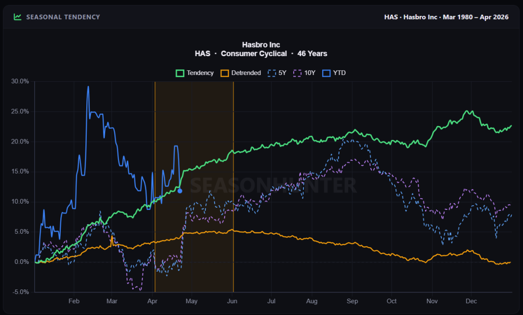
Il Pattern Scanner ha valutato decine di combinazioni di finestre per HAS e le ha classificate per score. La riga evidenziata, quella che ho tradato, è la finestra Long 04-03 → 06-02, 60 giorni, con uno score di 6119. È lo score più alto dell’intera lista. Lo scanner ti sta dicendo: questa è la finestra stagionale ricorrente più forte per questo strumento.
Ora analizziamo le statistiche.
Win rate del 77,8%. 35 vincite, 10 perdite, su 45 anni di dati.
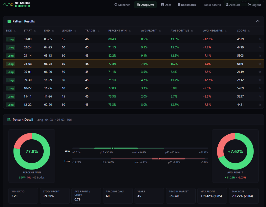
Non è un campione piccolo. 45 occorrenze storiche sono sufficienti per essere statisticamente significative. Tre volte su quattro in cui questo trade è stato aperto, si è chiuso in profitto. L’anno perdente su quattro è il rumore che accetti in cambio dell’edge.
Profitto medio: +7,62%
Ma le medie possono mentire. Quello che conta è la distribuzione. Guarda il breakdown per percentile:
| Metrica | Valore |
|---|---|
| Vincite p25 | +5.59% |
| Vincita mediana | +9.69% |
| Vincite p75 | +15.44% |
| Perdita mediana | -4.91% |
| Perdita p75 (peggior 25%) | -2.52% |
| Massimo profitto storico | +31.42% (1985) |
| Massima perdita storica | -13.27% (2004) |
L’asimmetria qui è esattamente ciò che vuoi vedere. La vincita mediana (+9.69%) è circa il doppio della perdita mediana (-4.91%). Anche il quartile più debole delle vincite (+5.59%) supera la perdita tipica. Questa è la forma di un edge autentico, non di una serie fortunata.
Win ratio: 2,23
Questo significa che i trade vincenti sono in media 2.23 volte più grandi dei trade perdenti. Combinato con un win rate del 77.8%, il valore atteso per trade è fortemente positivo. Non devi avere ragione ogni volta. Devi solo avere ragione la maggior parte delle volte e lasciare che la matematica lavori.
Profitto medio / Deviazione standard: 0,79
Pensalo come una metrica simile allo Sharpe per il pattern stagionale. Un valore sopra 0.5 è già solido. A 0.79, questo pattern ha un forte rapporto segnale/rumore — il rendimento medio è ampio rispetto alla variabilità anno per anno. L’edge è coerente, non guidato da una manciata di anni outlier.
Tempo a mercato: 16,4%
Questo è uno dei miei numeri preferiti dell’intera dashboard. Questo pattern richiede di essere esposti al rischio di mercato solo per il 16.4% dell’anno di calendario. Non resti nel trade a macinare rumore per 12 mesi. Sei dentro per una finestra definita di 60 giorni con un vento strutturale a favore, e poi fuori. Per il resto dell’anno, quel capitale è libero per altri setup.
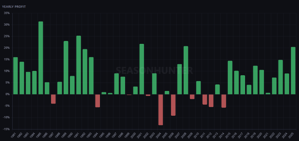
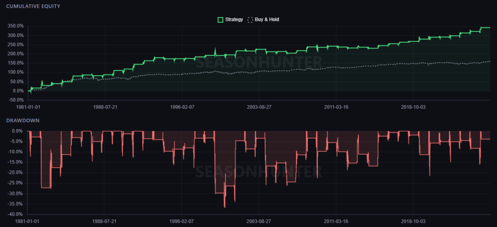
In effetti, se avessi tradato questo pattern stagionale in tutti gli anni, avrei ottenuto un grande profitto cumulativo.
Un’altra cosa degna di nota: guarda le altre righe nello scanner. La finestra March 14 → May 13 ha uno score di 5903 con un win rate dell’82.2%. La finestra January 9 → March 5 ha un win rate dell’80.4%. HAS non è un one-trick pony; ha una struttura stagionale ricorrente su più finestre durante l’anno. Questo è il tipo di strumento che vuoi in un portafoglio stagionale sistematico.
Tradare il segnale
La finestra del 3 aprile era quella in apertura imminente. I dati erano puliti. Ho aperto il trade.
Stock price at the time: ~$89.
Il setup che ho scelto era un Bull Put Spread:
| Parametro | Valore |
|---|---|
| Strategia | Bull Put Spread |
| Strike short put | $87.50 |
| Strike long put | $77.50 |
| Scadenza | June 18 |
| Premio incassato | $302 |
| Margine richiesto | ~$500 |
| Prezzo del titolo all’apertura | ~$89 |
La struttura è semplice: ho venduto la put $87.50 e comprato la put $77.50 come protezione. Il profitto massimo è il premio di $302 se HAS resta sopra $87.50 a scadenza. La perdita massima è limitata a $698 (l’ampiezza dello spread di $10 meno il premio incassato di $3.02).
Il punto chiave qui è il margine richiesto: meno di $500.
Quel numero conta. Ci torno tra poco.
Una settimana dopo: l’edge si manifesta
Entro l’8 aprile, circa una settimana dopo l’apertura del trade, HAS era passato da circa $89 a circa $93.80. Un movimento del +5.3% del sottostante.
Lo spread verticale, che avevo venduto per $302, si era ridotto a $214 di valore.
Questo è un guadagno di $88, o circa il 30% del profitto massimo, in circa 7 giorni di trading.
Ora, alcuni di voi stanno leggendo e pensando: $88? Tutto qui?
Giusto. In termini assoluti, non è una cifra che cambia la vita. Ma è qui che diventa interessante, ed è il motivo per cui le opzioni hanno un vantaggio intrinseco rispetto all’equity puro per questo tipo di operazione.
Il vantaggio delle opzioni: ritorno sul capitale
Facciamo il confronto correttamente.
Con $500 di capitale in un trade azionario, il 1° aprile avrei potuto comprare circa 5–6 azioni HAS a $89.
Diciamo che mi spingo a 6 azioni:
Capital deployed: 6 × $89 = $534
Value after move: 6 × $93.80 = $562.80
Profit: $28.80
Return on capital: ~5.4%
Ora guarda il trade in opzioni:
Margin required: ~$500
Profit captured (at +30% of max): $88
Return on capital: ~17.6%
Stesso capitale. Stessa scommessa direzionale. Stesso movimento del sottostante.
Options: +17.6%. Equity: +5.4%.
È un fattore di leva 3x sul capitale impiegato, senza assumere rischio illimitato. La struttura dello spread ti dà un pavimento rigido alle perdite. La posizione azionaria no.
Questo è ciò che intendo quando dico che le opzioni danno leva intrinseca con rischio controllato. Non stai puntando la casa. Stai usando il capitale in modo efficiente.
17 aprile: la decisione di uscita
Qui l’esecuzione conta più della teoria.
Entro il 17 aprile — 17 giorni dopo l’apertura del trade — HAS era ancora elevato. Lo spread verticale aveva continuato a ridursi e ora scambiava a $1.40.
Mettiamolo nel contesto:
| Valore | |
|---|---|
| Premio incassato all’apertura | $302 |
| Valore dello spread il 17 aprile | $140 |
| Profitto bloccato in caso di chiusura | $162 |
| Giorni trascorsi | 17 |
| Giorni alla scadenza | ~60 rimanenti |
La posizione aveva eroso circa il 54% del premio massimo in soli 17 giorni — meno di un quarto della vita del trade.
Ho chiuso.
Ho una regola per le strutture di vendita di premio, ed è semplice:
In questo caso:
· Tempo trascorso: 17 giorni su circa 78 totali = 22% della durata del trade
· Premio eroso: circa 54% del massimo
Ho raggiunto la soglia in anticipo. Il trade aveva fatto il suo lavoro.
La domanda a quel punto non è “quanto altro posso guadagnare?” È “perché sto ancora mantenendo rischio?”
Altri sessanta giorni di esposizione, attraverso earnings, eventi macro e spike di volatilità, per un potenziale ulteriore $140. Quella matematica non mi attrae. Avevo l’edge, l’ho catturato, sono andato avanti.
Questo è l’aspetto del trading sistematico: non avido, non emotivo, solo disciplinato.
Riassumiamo l’intero ciclo di vita:
| Data | Evento | P&L |
|---|---|---|
| 1 aprile | Apertura Bull Put Spread 87.5/77.5 giugno | +$302 incassati |
| 8 aprile | Spread a $214 (~30% di profitto) | +$88 non realizzati |
| 17 aprile | Chiusura posizione, spread a $140 | +$162 realizzati |
Final return on deployed capital: ~32.4% on less than $500 in 17 days.
Non cambia la vita. Ma è scalabile. E ripetibile, perché l’ingresso era basato su un edge statistico, non su una sensazione di pancia.
Il vero insegnamento operativo
Molti trader guardano i pattern stagionali e pensano: compra il titolo, cavalca il trend, vendi sul massimo.
Funziona. Ma le opzioni ti danno un set di strumenti diverso:
Rischio definito. Lo spread limita la perdita. Nessun dramma da stop-loss, nessun panico da gap-down. Conosci il worst case già all’ingresso.
Efficienza del capitale. Stai impiegando $500, non $5.000. Questo libera capitale per altri pattern stagionali, altre strategie, altri strumenti.
Time decay come alleato. Non hai bisogno che HAS esploda verso l’alto. Hai solo bisogno che resti sopra $87.50. Il tempo erode il valore dello spread sia che il titolo si muova sia che resti fermo.
Leva intrinseca. Lo stesso movimento del sottostante (+5.3%) ha prodotto 3x il ritorno sul capitale rispetto all’acquisto diretto di azioni.
Il position sizing resta importante? Assolutamente. Un singolo trade con $500 di margine non cambierà il tuo anno. Ma immagina di aver fatto questo lavoro di screening su 20 strumenti, identificato 8–10 setup stagionali di alta qualità e distribuito capitale sistematicamente su tutti. A quel punto la matematica inizia a comporsi.
Questa è l’architettura dietro SeasonHunter. Non un singolo trade — un portafoglio di edge.
Queste non sono narrative speculative; sono realtà di ciclo economico che si sono ripetute per decenni. Il pattern funziona perché i driver sottostanti persistono.
Una domanda per te
Voglio lasciarti con questa domanda:
Avrei dovuto tenere più a lungo? Lo spread era a $1.40, la scadenza era a 60 giorni. C’erano ancora $140 di premio da erodere. Alcuni trader avrebbero mantenuto la posizione. La mia regola diceva di chiudere.
Tu cosa avresti fatto?
Scrivimi e fammelo sapere, leggo davvero ogni messaggio. Queste discussioni plasmano il prossimo articolo.
Considerazioni finali
Gli edge stagionali non devono essere home run. Devono essere coerenti, ben dimensionati ed eseguiti in modo pulito.
HAS mi ha dato un movimento del sottostante del +5.3%, una struttura spread pulita e un’uscita disciplinata al 54% del profitto massimo in 17 giorni. Il capitale è tornato nel pool, pronto per il prossimo setup.
Questo è il gioco. Non eccitazione — ripetibilità.
Se non hai ancora esplorato SeasonHunter, inizia con la prova gratuita di 2 settimane — nessuna carta di credito richiesta. Esegui lo screener, filtra per la tua finestra di ingresso preferita e soglia di win rate, e guarda cosa fa emergere il dato. Il pattern HAS che ho tradato qui è esattamente il tipo di setup che produce ogni singolo mese su migliaia di strumenti.
L’edge è nei dati. L’esecuzione dipende da te.
→ Inizia la tua prova gratuita su SeasonHunterQuesto è il mindset dietro The Quantitative Edge — idee semplici, implementate in modo pulito, che scalano in strumenti potenti per il trading data-driven.
Statemi bene!
Avvertenza importante — Non è consulenza finanziaria
Importante: né questo articolo né il tool SeasonHunter forniscono consulenza finanziaria, consulenza di investimento, raccomandazioni di trading o qualsiasi altro tipo di servizio finanziario regolamentato.
Tutti i contenuti, i dati, gli esempi operativi e le analisi presentate sono esclusivamente a scopo informativo e non costituiscono in alcun modo un invito a comprare, vendere o detenere strumenti finanziari.
I pattern stagionali osservati nel passato non rappresentano una garanzia di risultati futuri. Ogni decisione di investimento deve essere presa in modo autonomo e, se necessario, con il supporto di un consulente finanziario qualificato.
Il trading comporta rischi significativi, inclusa la possibile perdita del capitale investito.
The Bull Put Spread Trade on Seasonal Edge
Description
Last month, I walked you through McDonald’s seasonal edge: 56 years of data, a 73% win rate, and a clear entry window from late March to early May. The theory was there. The data was there. But theory only gets you so far.
This time I want to show you something different. A real trade. Open to close. Numbers included.
The ticker is Hasbro (HAS). The instrument is a bull put spread. The result? Closed in 17 days with ~54% of the maximum profit captured, and a return on capital that no equity position could have matched with the same money.
Let me walk you through it.
The Tool Behind the Trade: SeasonHunter
Before I get into the trade itself, let me spend a minute on the tool that surfaced it, because without it, HAS wouldn’t have been on my radar at all.
SeasonHunter is a stock seasonality screener built specifically for this kind of systematic work. It tracks over 3,000 financial instruments — equities, ETFs, sector funds — and evaluates 365 calendar days of potential entry windows against 30+ years of price history. The output isn’t a vague “this stock tends to go up in spring.” It’s a ranked, filterable list of patterns with hard numbers behind each one.
Here’s what the workflow looks like in practice:
Step 1 — Set your time horizon. You pick an entry date and a window length. A week, a month, longer; whatever matches your strategy.
Step 2 — Filter the market. You narrow by sector, Long or Short directional bias, and minimum historical win rate. In my April screening, I filtered for Long setups opening in the first week of April with a win rate above 65%.
Step 3 — Inspect the pattern. For every result, SeasonHunter shows you the full picture: the seasonal tendency chart, a year-by-year P&L breakdown, cumulative equity curve with drawdown overlay, and monthly/yearly win-rate heatmaps. You see exactly how durable the edge is, not just the average, but the distribution.
Step 4 — Trade with conviction. You enter only what the data supports. No guesswork, no narratives. Just decades of repeating behaviour.
What I particularly use is the Pattern Scanner (available in the Premium tier). Rather than testing a single entry date, it evaluates thousands of window combinations for a given instrument and ranks them by statistical robustness. It’s how I found both MCD and HAS — the scanner surfaces the strongest window for each month of the year, so I always know where the next edge is before the calendar turns.
The best seasonal trades combine a high win rate, a meaningful average gain, and robust metrics. This creates consistent performance across years — not just a handful of outlier results.
If you want to explore it yourself, SeasonHunter offers a 2-week free trial with full Pro access, no credit card required. It’s how I’d suggest you start: run the screener, find a pattern, and paper trade it before committing real capital. The workflow becomes intuitive very quickly.
→ Try SeasonHunter free for 2 weeksThe Setup: April 1st Screening
On April 1st, I ran my seasonal screening using SeasonHunter. HAS has come up with a strong recurring pattern; historically, the stock tends to drift upward during this specific window. The signal was clean: directional bias, defined seasonality, and clear entry timing.
The Pattern Scanner has evaluated dozens of window combinations for HAS and ranked them by score. The highlighted row, the one I traded, is the Long 04-03 → 06-02, 60-day window, with a score of 6119. That’s the highest score on the entire list. The scanner is telling you: this is the strongest recurring seasonal window for this instrument.
Now let’s unpack the statistics.
77.8% win rate. 35 wins, 10 losses, across 45 years of data.
That’s not a small sample. 45 historical occurrences are enough to be statistically meaningful. Three out of every four times this trade was opened, it closed profitably. The one losing year in four is the noise you accept in exchange for the edge.
Average profit: +7.62%
But averages can lie. What matters is the distribution. Look at the percentile breakdown:
| Metric | Value |
|---|---|
| Win p25 | +5.59% |
| Win median | +9.69% |
| Win p75 | +15.44% |
| Loss median | -4.91% |
| Loss p75 (worst 25%) | -2.52% |
| Max historical profit | +31.42% (1985) |
| Max historical loss | -13.27% (2004) |
The asymmetry here is what you want to see. The median win (+9.69%) is roughly double the median loss (-4.91%). Even the weakest quartile of wins (+5.59%) outperforms the typical loss. This is the shape of a genuine edge, not a lucky streak.
Win ratio: 2.23
This means winning trades are on average 2.23x larger than losing trades. Combined with a 77.8% win rate, the expected value per trade is strongly positive. You don’t need to be right every time. You just need to be right most of the time and let the math work.
Avg Profit / StDev: 0.79
Think of this as a Sharpe-like metric for the seasonal pattern. A value above 0.5 is already solid. At 0.79, this pattern has a strong signal-to-noise ratio — the average return is large relative to the year-to-year variability. The edge is consistent, not driven by a handful of outlier years.
Time in market: 16.4%
This is one of my favourite numbers on the entire dashboard. This pattern only requires you to be exposed to market risk for 16.4% of the calendar year. You’re not sitting in the trade grinding through 12 months of noise. You’re in for a defined 60-day window with a structural tailwind, and out. The rest of the year, that capital is free for other setups.
Indeed, if I had traded this seasonal pattern over all the years, I would have gained a great cumulative profit.
One more thing worth noting: look at the other rows in the scanner. The March 14 → May 13 window scores 5903 with an 82.2% win rate. The January 9 → March 5 window has an 80.4% win rate. HAS isn’t a one-trick pony; it has recurring seasonal structure across multiple windows throughout the year. That’s the kind of instrument you want in a systematic seasonal portfolio.
Trading the Signal
The April 3 window was the one opening imminently. The data was clean. I opened the trade.
Stock price at the time: ~$89.
The setup I chose was a Bull Put Spread:
| Parameter | Value |
|---|---|
| Strategy | Bull Put Spread |
| Short Put Strike | $87.50 |
| Long Put Strike | $77.50 |
| Expiration | June 18 |
| Premium Collected | $302 |
| Margin Required | ~$500 |
| Stock Price at Open | ~$89 |
The structure is simple: I sold the $87.50 put and bought the $77.50 put as protection. Maximum profit is the $302 premium if HAS stays above $87.50 at expiration. Maximum loss is capped at $698 (the $10 spread width minus the $3.02 premium collected).
The key here is the margin required: less than $500.
That number matters. I’ll come back to it.
One Week Later: The Edge Shows Up
By April 8th, roughly one week after opening the trade, HAS had moved from ~$89 to ~$93.80. A +5.3% move in the underlying.
The vertical spread, which I had sold for $302, had deflated to $214 in value.
That’s an $88 gain, or roughly 30% of the maximum profit, in about 7 trading days.
Now, some of you are reading that and thinking: $88? That’s it?
Fair. In absolute terms, it’s not a life-changing number. But here’s where it gets interesting, and why options have an intrinsic advantage over pure equity for this kind of play.
The Options Advantage: Return on Capital
Let’s do the comparison properly.
With $500 of capital in a stock trade, on April 1st, I could buy approximately 5–6 shares of HAS at $89.
Let’s say I stretch to 6 shares:
Capital deployed: 6 × $89 = $534
Value after move: 6 × $93.80 = $562.80
Profit: $28.80
Return on capital: ~5.4%
Now look at the options trade:
Margin required: ~$500
Profit captured (at +30% of max): $88
Return on capital: ~17.6%
Same capital. Same directional bet. Same underlying move.
Options: +17.6%. Equity: +5.4%.
That’s a 3x leverage factor on deployed capital, without taking on unlimited risk. The spread structure gives you a hard floor on losses. The equity position doesn’t.
This is what I mean when I say options give you intrinsic leverage with controlled risk. You’re not betting the house. You’re using capital efficiently.
April 17th: The Exit Decision
Here’s where execution matters more than theory.
By April 17th — 17 days after opening the trade — HAS was still elevated. The vertical spread had continued to deflate and was now trading at $1.40.
Let me put that in context:
| Value | |
|---|---|
| Premium collected at open | $302 |
| Spread value on April 17 | $140 |
| Profit locked in if closed | $162 |
| Days elapsed | 17 |
| Days to expiration | ~60 remaining |
The position had eroded roughly 54% of the maximum premium in just 17 days — less than a quarter of the way through the life of the trade.
I closed it.
I have a rule for premium-selling structures, and it’s simple:
In this case:
· Time elapsed: 17 days out of ~78 total = 22% of the trade’s duration
· Premium eroded: ~54% of maximum
I hit the threshold early. The trade had done its job.
The question at that point isn’t “how much more can I make?” It’s “Why am I still holding risk?”
Sixty more days of exposure, through earnings, macro events, and volatility spikes, for a potential additional $140. That math doesn’t appeal to me. I had the edge, I captured it, I moved on.
This is what systematic trading looks like: not greedy, not emotional, just disciplined.
Let me summarise the complete lifecycle:
| Date | Event | P&L |
|---|---|---|
| April 1 | Open Bull Put Spread 87.5/77.5 June | +$302 collected |
| April 8 | Spread at $214 (~30% profit) | +$88 unrealized |
| April 17 | Close position, spread at $140 | +$162 realized |
Final return on deployed capital: ~32.4% on less than $500 in 17 days.
Not life-changing. But scalable. And repeatable, because the entry was based on a statistical edge, not a gut feeling.
The Real Takeaway
A lot of traders look at seasonal patterns and think: buy the stock, ride the trend, sell at the top.
That works. But options give you a different set of tools:
Defined risk. The spread caps your loss. No stop-loss drama, no gap-down panic. You know the worst case at entry.
Capital efficiency. You’re deploying $500, not $5,000. That frees capital for other seasonal patterns, other strategies, other instruments.
Time decay as an ally. You don’t need HAS to skyrocket. You just need it to stay above $87.50. Time erodes the spread’s value whether the stock moves or stands still.
Intrinsic leverage. Same underlying move (+5.3%) delivered 3x the return on capital compared to buying shares outright.
Is position sizing still important? Absolutely. One trade at a $500 margin isn’t going to change your year. But imagine you’ve done this screening work across 20 instruments, identified 8–10 high-quality seasonal setups, and deployed capital systematically across all of them. Now the math starts to compound.
That’s the architecture behind SeasonHunter. Not a single trade — a portfolio of edges.
These aren’t speculative narratives; they’re business cycle realities that have repeated for decades. The pattern works because the underlying drivers persist.
A Question for You
I want to leave you with this:
Should I have held longer? The spread was at $1.40, expiration was 60 days away. There was $140 of premium still to erode. Some traders would have held. My rule said close.
What would you have done?
Write to me and let me know, I genuinely read every message. These discussions shape the next article.
Final Thoughts
Seasonal edges don’t need to be home runs. They need to be consistent, well-sized, and executed cleanly.
HAS gave me a +5.3% underlying move, a clean spread structure, and a disciplined exit at 54% of maximum profit in 17 days. The capital returned to the pool, ready for the next setup.
That’s the game. Not excitement — repeatability.
If you haven’t explored SeasonHunter yet, start with the free 2-week trial — no credit card needed. Run the screener, filter by your preferred entry window and win rate threshold, and see what the data surfaces. The HAS pattern I traded here is exactly the kind of setup it produces every single month across thousands of instruments.
The edge is in the data. Execution is up to you.
→ Start your free trial at SeasonHunterThis is the mindset behind The Quantitative Edge — simple ideas, implemented cleanly, that scale into powerful tools for data-driven trading.
Statemi bene!
Important Notice — Not financial advice
Important: neither this article nor the SeasonHunter tool provides investment advice, financial advice, trading advice, or any other type of regulated financial service.
All content, data, examples, screener results, and analytics presented are for informational purposes only and do not constitute a recommendation to buy, sell, or hold any financial instrument.
Past seasonal patterns are not a guarantee of future results. You should always conduct your own research and consult a qualified financial adviser before making any investment decision.
Trading involves risk, including the possible loss of principal.
