
Our work is fascinating, complex, and closely tied to uncertainty. We’re talking about those who operate in financial markets, regardless of the techniques they use, whether they are discretionary, systematic, or aided by new AI technologies. Beyond the allure that some of these approaches might bring to our perception, it is always the medium- and long-term results that determine the validity of these methodologies. Observing results over the medium and long term should help, depending on the technique used, to distinguish “lucky” outcomes that might be linked to a single, non-repeatable good intuition (think of buying assets and holding them in a portfolio for years, like a buy-and-hold strategy). A concrete example includes those who purchased stocks during expansion phases like the dot-com boom at the end of the last century or post-subprime crisis, those who held penny stocks for a decade that then soared, or cryptocurrencies in the last ten years. Far be it from us to diminish the value of such investments (the results speak for themselves); here, we are not looking to investigate a few fortunate occurrences but rather a statistically observable progression of repetitive actions that form a method.
But what exactly are we trying to investigate?
We want to understand if and how it is possible to generate value over time in financial markets by identifying and exploiting statistically detectable patterns, blending a systematic approach with an AI-driven one. Simply put, we want to know if there exists a competitive edge intrinsically tied to financial data.
Let’s be clear. For those like us who have been working on machine learning with large volumes of financial data for years, it is an ongoing challenge to measure these data’s ability to predict the future. And this capability, in 2024, must be comparable to that of an operator making discretionary decisions. The more astute might argue that a discretionary operator could make operational decisions not only based on observed data but also on context and personal experience, referring to data that may seem unrelated to the problem at hand. They could change behavior depending on the season, their mental and physical state, upcoming elections (like the U.S. elections next week), or any other “disturbing element.” However, all these factors, in their complexity, characterize data that could be used (or not) by a machine learning model (except, partially, for the psychophysical state).
But is it really possible to synthesize all these data, and what kind of uncertainty are we talking about?
To avoid any misunderstanding, I’ll say right away that we are far from perfect prediction; rather, we’re talking about “statistical forecasting.” However, even adding a few percentage points of probability in your favor can make a huge difference, as anyone operating in financial markets knows well. Modern hedge funds are well aware of this, investing increasingly substantial capital in new technologies.
But what kind of predictions are we talking about?
Everyone immediately thinks of direct price prediction (or at least percentage variation), and it must be said that there are some very interesting results from this perspective (we’ll discuss this in a future article). However, what is often achievable is more subtle, yet equally useful. One such application of machine learning (which we have been working on for years) is the clustering of volatility dynamics.
Imagine being an options trader with a weekly or daily forecast of the expected volatility on your instruments. This would add a third key to historical volatility and implied volatility, with measurable advantages within a strategy (future articles will also cover this topic). Or imagine being a trading system designer wanting to use such information to filter signals generated by your machines. This would indeed constitute a significant competitive advantage.
Now there are three elements to consider when designing predictive systems: data, machine learning models, and time. These variables are often interlinked and can be decisive in achieving the final result.
The Data
This refers to the database, appropriately processed, that forms the input for our systems. Referring to regulated markets, it may contain price data, volume data, macroeconomic data (such as interest rates or the unemployment rate), alternative data linked to highway traffic, lunar phases, solar storms, natural disasters, sentiment curves of major opinion leaders, and much more (only research on their actual effectiveness can guide their use). Data represents the most crucial and decisive variable for the success of our experiment. If the data lacks predictive elements for the variable we aim to forecast, the entire investigation will fail, presenting results akin to random choices.
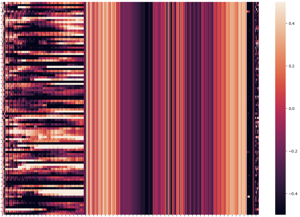
In the figure, you can observe the temporal sampling of a well-processed dataset, with data related to an equity basket (on the left) and “contextual” data (on the right) to guide a general decision-making process.
The Models
Machine learning models can have widely varying characteristics, using linear or non-linear functions with increasing complexity, depending on the problem to be solved. These range from Linear Regression, Logistic Regression, Decision Trees, Random Forest, Support Vector Machines, ensemble methods (such as XGBoost, LightGBM, CatBoost), to Stacked Deep Neural Networks (like MLP, CNN, LSTM, etc.). Generally, the model’s importance, once the correct category is appropriately associated with the variable to be predicted, is less significant compared to the quality of the data used.
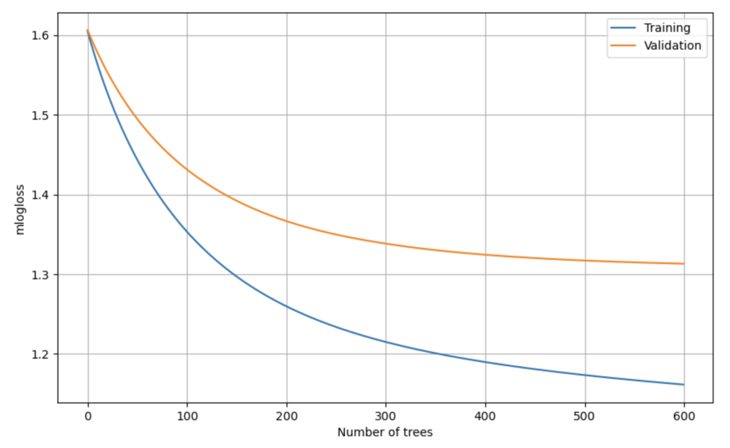
In the figure, we can observe the learning curve of an ensemble algorithm (based on decision trees) on training data (in-sample, shown in blue) and on unknown data (out-of-sample, shown in orange). What emerges is a good ability to improve decisions based on input data. This is the first element to consider before proceeding with using a model, even before evaluating its real-world results.
Time
Time is the most limiting factor. This includes processing and training time, but also execution time. The larger a dataset becomes, the more we shift from a classic machine learning problem to one of big data analysis, which inevitably impacts available resources. Although technology (especially hardware) helps us with these challenges, modern techniques in “dimensionality reduction” and “feature selection” significantly reduce processing time.
Volatility Forecasting
In this article, we aim to introduce one of the applications we have been working on for years, which represents one of the most effective predictors that can be developed by dynamically training our proprietary machine learning model: volatility clustering prediction.
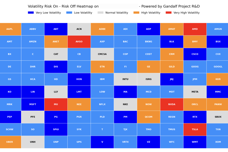
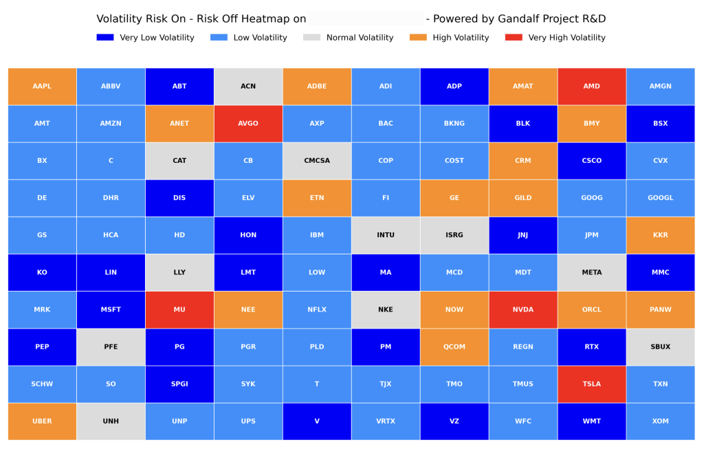
In the example below, you can see a heatmap that displays the five volatility clusters for the top 100 S&P 500 stocks by market capitalization on a specific date:
Dark Blue: A significant decrease in volatility is forecasted.
Light Blue: A moderate decrease in volatility is expected.
Ice Gray: Volatility is expected to remain relatively unchanged around the average.
Orange: A moderate increase in volatility is predicted.
Red: A significant increase in volatility is forecasted.
The same outputs can, of course, be presented with greater detail: for example, by associating a probability with each class (imagine the implications for the position sizing in a composite asset allocation system aimed at minimizing expected risk).
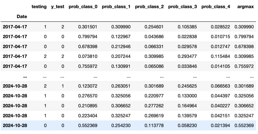
The table above associates the probability with which the machine assigns each class: in the last row (corresponding to a specific asset), for instance, Class 0, the one with the highest confidence, is recognized with a 55% probability.
However, we need a quantitative method to unambiguously assess the quality of our prediction.
Below is a Classification Report (from one of the intermediate development trials, which will be further refined and standardized across classes) that assigns a specific Accuracy to each class.
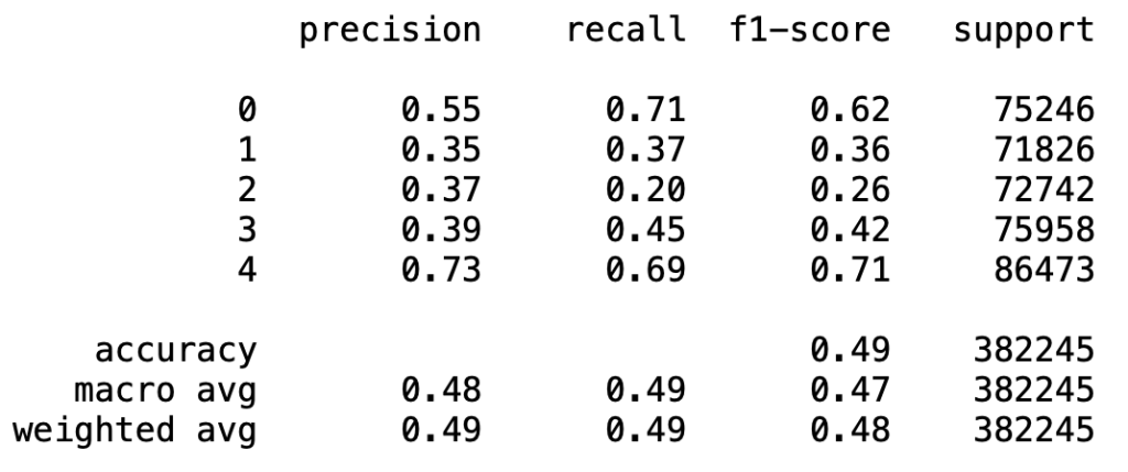
Class Evaluation:
Class 0 performs decently, with a precision of 0.55 (55%) and a recall of 0.71, resulting in an F1-score of 0.62. This indicates that the model is reasonably effective in identifying samples of this class.
Class 4 also shows good performance, with a precision of 0.73 (73%), a recall of 0.69, and an F1-score of 0.71, suggesting that the model predicts this class accurately.
Classes 1, 2, and 3 have lower precision, recall, and F1-scores, with Class 2 particularly problematic (F1-score of 0.26). This suggests that the model struggles to correctly distinguish samples in these classes, likely due to overlapping features or difficulty in separating them.
Overall Evaluation:
• Accuracy: The overall accuracy is 0.49, indicating that the model correctly predicts about 49% of the samples.
• Macro Average: The macro F1-score average is 0.47.
• Weighted Average: The weighted F1-score is 0.48, taking into account the support of each class. This value, slightly higher than the macro average, indicates that the model performs better on more frequent classes but has difficulty with the less common ones.
To determine whether these results are better than random classification, let’s compare the model’s performance with what we’d expect by chance.
Random Baseline:
For a classification problem with five classes, a purely random classifier would have an accuracy of approximately 20% (1 out of 5 classes). Precision, recall, and F1-scores would be around 0.20 for each class if predictions were random and evenly balanced.
Observed Results:
The model’s overall accuracy of 0.49 is more than double the random baseline of 0.20. This suggests that the model captures some meaningful information in the data, rather than just making random choices.
Classes 0 and 4 show precision, recall, and F1-scores significantly higher than expected for random classification (with Class 4 having the highest F1-score of 0.71). This indicates that the model successfully distinguishes these classes.
Classes 1, 2, and 3 show lower performance, with F1-scores between 0.26 and 0.42. While these scores are not ideal, they are still above 0.20 (the expected level for random predictions), suggesting that the model performs better than random classification even for these harder-to-distinguish classes. The model’s difficulty with these classes may stem from feature overlap, class imbalance, or insufficiently distinctive features. Nevertheless, the model still captures some structure in the data.
This trial-and-error approach will continue until the model reliably presents data that is genuinely useful.
But what is the impact of an average accuracy of 49% at an operational level?
In one of the upcoming articles, we’ll see these predictions in action to manage asset allocation risk and to filter quantitative trading and investing strategies.
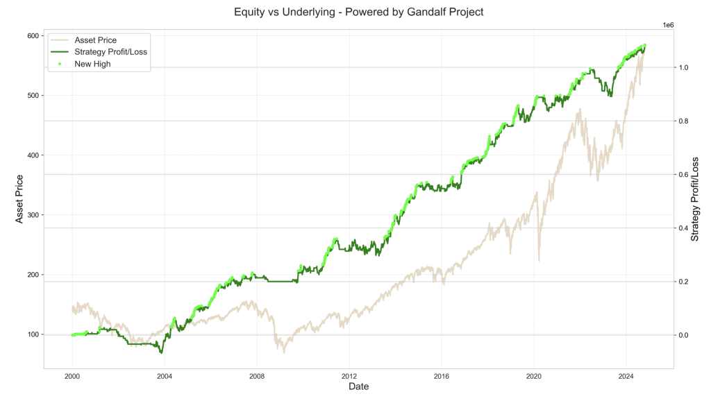
All tables and analyses presented in this article were created using Python code. The skills required for these tasks are explored in depth within Gandalf Project’s two educational accelerators: Python Academy and Machine Learning Academy.
Anyone interested in diving deeper into these topics or seeking information on available forecasting services (price, volatility, and market scenarios) can contact us at info@gandalfproject.com.
Giovanni Trombetta
Founder – Head of R&D
Gandalf Project
